[고체역학] 모어 원 그리기

MATLAB으로 모어 원을 그려보자. 손으로 그리면 원이 예쁘게 안 그려져서 답답해서 만들어 보았다.

 

 모어 원에 대한 자세한 설명이 필요하면 아래 글을 참고하면 좋겠다.

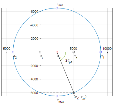
모어 원 (Mohr's Circle)

 

그림 1. 모어 원을 간단하게 그려보자

Mohrs_Circle.m

0.00MB

%% clear
clear all
clc

%% Stress state
sigma_x = 5000;
sigma_y = 0;
sigma_xy = 6000;

% sigma_x = 1800;
% sigma_y = 4200;
% sigma_xy = -4000;

% sigma_x = -4000;
% sigma_y = 0;
% sigma_xy = -4000;

%% Calculation
% Average stress
sigma_m = (sigma_x + sigma_y)/2;
% Radius of Mohr's circle
R = sqrt(0.25*(sigma_x-sigma_y)^2 + sigma_xy^2);

% Principal stresses and max & min shear stresses.
sigma_1 = sigma_m + R;
sigma_2 = sigma_m - R;
tau_max = R;
tau_min = -R;

% Principal directions
theta_p1 = 0.5*atan2(2*sigma_xy, sigma_x-sigma_y);
theta_s1 = -0.5*atan2(sigma_x-sigma_y, 2*sigma_xy);

theta_p2 = theta_p1 + pi/2;
theta_s2 = theta_s1 + pi/2;

% Mohr's circle
center_x = sigma_m;
center_y = 0;
angles = linspace(0, 2*pi, 360);
x = R*cos(angles);
y = R*sin(angles);

%% Plot
figure(1)
% Plot circle
plot(x+center_x, y+center_y);
grid on
hold on
axis equal
ax = gca;
ax.XAxisLocation = 'origin';
ax.YAxisLocation = 'origin';
% Reverse Y axis
set(gca, 'Ydir', 'reverse');
% set(gca, 'XTick', [-10000:2000:10000]);
% xlim([sigma_m - 1.2*R, sigma_m + 1.2*R]);
% ylim([-R*1.2, R*1.2]);

% Plot points an texts
plot(sigma_x, 0, 'o', 'color', 'black')
text(sigma_x, R*0.10, '\sigma_x');
plot(sigma_y, 0, 'o', 'color', 'black')
text(sigma_y, R*0.10, '\sigma_y');
plot(sigma_x, sigma_xy, 'o', 'color', 'black')
text(sigma_x, sigma_xy + R*0.10, '(\sigma_x, \sigma_{xy})');
line([sigma_m, sigma_x], [0, sigma_xy], 'color', 'black', 'LineStyle', '-');
line([0, sigma_x], [sigma_xy, sigma_xy], 'color', 'black', 'LineStyle', '--');

% Draw angle
if theta_p1 > 0
    theta = -2*theta_p1:1/360:0;
else
    theta = 0:1/360:-2*theta_p1;
end
r = R*0.2;
xx = r*cos(theta);
yy = r*sin(-theta);

plot(xx+sigma_m, yy)
text(r+sigma_m,r,'2\theta_{p1}')

% Plot calculated points and texts 
plot(sigma_m, 0, 'o', 'color', 'r')
text(sigma_m, R*0.10, '\sigma_m');
plot(sigma_1, 0, 'o', 'color', 'b')
text(sigma_1, R*0.10, '\sigma_1');
plot(sigma_2, 0, 'o', 'color', 'b')
text(sigma_2, R*0.10, '\sigma_2');
plot(sigma_m, tau_max, 'o', 'color', 'b')
text(sigma_m, tau_max+R*0.10, '\tau_{max}');
line([sigma_m, sigma_m], [0, tau_max], 'color', 'black', 'LineStyle', '--');
plot(sigma_m, tau_min, 'o', 'color', 'b')
text(sigma_m, tau_min-R*0.10, '\tau_{min}');
line([sigma_m, sigma_m], [0, tau_min], 'color', 'black', 'LineStyle', '--');

%% Print results
fprintf('sigma_x\t= %+.2f,\ttheta_1 = %+3.2f degrees\n', sigma_x, 0)
fprintf('sigma_y\t= %+.2f,\ttheta_2 = %+3.2f degrees\n', sigma_y, 90)
fprintf('\n')
fprintf('sigma_m\t= %+.2f\n', sigma_m);
fprintf('Radius\t= %+.2f\n', R);
fprintf('\n')
fprintf('sigma_1\t= %+.2f,\ttheta_p1 = %+.2f degrees\n', sigma_1, rad2deg(theta_p1));
fprintf('sigma_2\t= %+.2f,\ttheta_p2 = %+.2f degrees\n', sigma_2, rad2deg(theta_p2));
fprintf('tau_max\t= %+.2f,\ttheta_s1 = %+.2f degrees\n', tau_max, rad2deg(theta_s1));
fprintf('tau_min\t= %+.2f,\ttheta_s2 = %+.2f degrees\n', tau_min, rad2deg(theta_s2));